电子产品世界

　　2.3 创建一个简单的一层神经网络

　　神经网络最简单的形式是一层线性全连接神经网络(FCNN， Fully Connected Neural Network)。 在数学上它由一个矩阵乘法组成。

　　最好是在Tensorflow中从这样一个简单的NN开始，然后再去研究更复杂的神经网络。 当我们研究那些更复杂的神经网络的时候，只是图的模型(步骤2)和权重(步骤3)发生了改变，其他步骤仍然保持不变。

　　我们可以按照如下代码制作一层FCNN：

　　image_width = mnist_image_width

　　image_height = mnist_image_height

　　image_depth = mnist_image_depth

　　num_labels = mnist_num_labels

　　#the dataset

　　train_dataset = mnist_train_dataset

　　train_labels = mnist_train_labels

　　test_dataset = mnist_test_dataset

　　test_labels = mnist_test_labels

　　#number of iterations and learning rate

　　num_steps = 10001

　　display_step = 1000

　　learning_rate = 0.5

　　graph = tf.Graph()

　　with graph.as_default():

　　#1) First we put the input data in a Tensorflow friendly form.

　　tf_train_dataset = tf.placeholder(tf.float32, shape=(batch_size, image_width, image_height, image_depth))

　　tf_train_labels = tf.placeholder(tf.float32, shape = (batch_size, num_labels))

　　tf_test_dataset = tf.constant(test_dataset, tf.float32)

　　#2) Then, the weight matrices and bias vectors are initialized

　　#as a default, tf.truncated_normal() is used for the weight matrix and tf.zeros() is used for the bias vector.

　　weights = tf.Variable(tf.truncated_normal([image_width image_height image_depth, num_labels]), tf.float32)

　　bias = tf.Variable(tf.zeros([num_labels]), tf.float32)

　　#3) define the model:

　　#A one layered fccd simply consists of a matrix multiplication

　　def model(data, weights, bias):

　　return tf.matmul(flatten_tf_array(data), weights) + bias

　　logits = model(tf_train_dataset, weights, bias)

　　#4) calculate the loss, which will be used in the optimization of the weights

　　loss = tf.reduce_mean(tf.nn.softmax_cross_entropy_with_logits(logits=logits, labels=tf_train_labels))

　　#5) Choose an optimizer. Many are available.

　　optimizer = tf.train.GradientDescentOptimizer(learning_rate).minimize(loss)

　　#6) The predicted values for the images in the train dataset and test dataset are assigned to the variables train_prediction and test_prediction.

　　#It is only necessary if you want to know the accuracy by comparing it with the actual values.

　　train_prediction = tf.nn.softmax(logits)

　　test_prediction = tf.nn.softmax(model(tf_test_dataset, weights, bias))

　　with tf.Session(graph=graph) as session:

　　tf.global_variables_initializer().run()

　　print('Initialized')

　　for step in range(num_steps):

　　_, l, predictions = session.run([optimizer, loss, train_prediction])

　　if (step % display_step == 0):

　　train_accuracy = accuracy(predictions, train_labels[:, :])

　　test_accuracy = accuracy(test_prediction.eval(), test_labels)

　　message = "step {:04d} : loss is {:06.2f}, accuracy on training set {:02.2f} %, accuracy on test set {:02.2f} %".format(step, l, train_accuracy, test_accuracy)

　　print(message)

　　>>> Initialized

　　>>> step 0000 : loss is 2349.55, accuracy on training set 10.43 %, accuracy on test set 34.12 %

　　>>> step 0100 : loss is 3612.48, accuracy on training set 89.26 %, accuracy on test set 90.15 %

　　>>> step 0200 : loss is 2634.40, accuracy on training set 91.10 %, accuracy on test set 91.26 %

　　>>> step 0300 : loss is 2109.42, accuracy on training set 91.62 %, accuracy on test set 91.56 %

　　>>> step 0400 : loss is 2093.56, accuracy on training set 91.85 %, accuracy on test set 91.67 %

　　>>> step 0500 : loss is 2325.58, accuracy on training set 91.83 %, accuracy on test set 91.67 %

　　>>> step 0600 : loss is 22140.44, accuracy on training set 68.39 %, accuracy on test set 75.06 %

　　>>> step 0700 : loss is 5920.29, accuracy on training set 83.73 %, accuracy on test set 87.76 %

　　>>> step 0800 : loss is 9137.66, accuracy on training set 79.72 %, accuracy on test set 83.33 %

　　>>> step 0900 : loss is 15949.15, accuracy on training set 69.33 %, accuracy on test set 77.05 %

　　>>> step 1000 : loss is 1758.80, accuracy on training set 92.45 %, accuracy on test set 91.79 %

　　在图中，我们加载数据，定义权重矩阵和模型，从分对数矢量中计算损失值，并将其传递给优化器，该优化器将更新迭代“num_steps”次数的权重。

　　在上述完全连接的NN中，我们使用了梯度下降优化器来优化权重。然而，有很多不同的优化器可用于Tensorflow。 最常用的优化器有GradientDescentOptimizer、AdamOptimizer和AdaGradOptimizer，所以如果你正在构建一个CNN的话，我建议你试试这些。

　　Sebastian Ruder有一篇不错的博文介绍了不同优化器之间的区别，通过这篇文章，你可以更详细地了解它们。

　　2.4 Tensorflow的几个方面

　　Tensorflow包含许多层，这意味着可以通过不同的抽象级别来完成相同的操作。这里有一个简单的例子，操作

　　logits = tf.matmul(tf_train_dataset, weights) + biases，

　　也可以这样来实现

　　logits = tf.nn.xw_plus_b(train_dataset, weights, biases)。

　　这是layers API中最明显的一层，它是一个具有高度抽象性的层，可以很容易地创建由许多不同层组成的神经网络。例如，conv_2d()或fully_connected()函数用于创建卷积和完全连接的层。通过这些函数，可以将层数、过滤器的大小或深度、激活函数的类型等指定为参数。然后，权重矩阵和偏置矩阵会自动创建，一起创建的还有激活函数和丢弃正则化层(dropout regularization laye)。

　　例如，通过使用 层API，下面这些代码：

　　import Tensorflow as tf

　　w1 = tf.Variable(tf.truncated_normal([filter_size, filter_size, image_depth, filter_depth], stddev=0.1))

　　b1 = tf.Variable(tf.zeros([filter_depth]))

　　layer1_conv = tf.nn.conv2d(data, w1, [1, 1, 1, 1], padding='SAME')

　　layer1_relu = tf.nn.relu(layer1_conv + b1)

　　layer1_pool = tf.nn.max_pool(layer1_pool, [1, 2, 2, 1], [1, 2, 2, 1], padding='SAME')

　　可以替换为

　　from tflearn.layers.conv import conv_2d, max_pool_2d

　　layer1_conv = conv_2d(data, filter_depth, filter_size, activation='relu')

　　layer1_pool = max_pool_2d(layer1_conv_relu, 2, strides=2)

　　可以看到，我们不需要定义权重、偏差或激活函数。尤其是在你建立一个具有很多层的神经网络的时候，这样可以保持代码的清晰和整洁。

　　然而，如果你刚刚接触Tensorflow的话，学习如何构建不同种类的神经网络并不合适，因为tflearn做了所有的工作。

　　因此，我们不会在本文中使用层API，但是一旦你完全理解了如何在Tensorflow中构建神经网络，我还是建议你使用它。

　　2.5 创建 LeNet5 卷积神经网络

　　下面我们将开始构建更多层的神经网络。例如LeNet5卷积神经网络。

　　LeNet5 CNN架构最早是在1998年由Yann Lecun(见论文)提出的。它是最早的CNN之一，专门用于对手写数字进行分类。尽管它在由大小为28 x 28的灰度图像组成的MNIST数据集上运行良好，但是如果用于其他包含更多图片、更大分辨率以及更多类别的数据集时，它的性能会低很多。对于这些较大的数据集，更深的ConvNets(如AlexNet、VGGNet或ResNet)会表现得更好。

　　但由于LeNet5架构仅由5个层构成，因此，学习如何构建CNN是一个很好的起点。

　　Lenet5架构如下图所示：

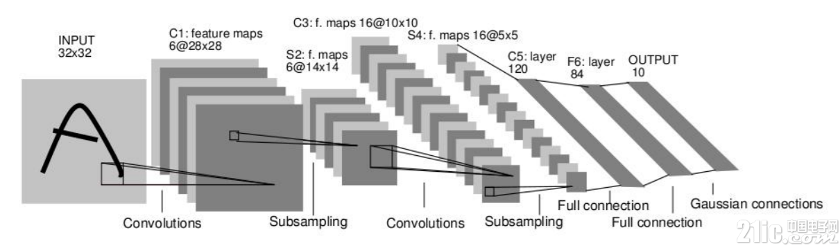
　　我们可以看到，它由5个层组成：

　　第1层：卷积层，包含S型激活函数，然后是平均池层。

　　第2层：卷积层，包含S型激活函数，然后是平均池层。

　　第3层：一个完全连接的网络(S型激活)

　　第4层：一个完全连接的网络(S型激活)

　　第5层：输出层

　　这意味着我们需要创建5个权重和偏差矩阵，我们的模型将由12行代码组成(5个层 + 2个池 + 4个激活函数 + 1个扁平层)。

　　由于这个还是有一些代码量的，因此最好在图之外的一个单独函数中定义这些代码。

　　LENET5_BATCH_SIZE = 32

　　LENET5_PATCH_SIZE = 5

　　LENET5_PATCH_DEPTH_1 = 6

　　LENET5_PATCH_DEPTH_2 = 16

　　LENET5_NUM_HIDDEN_1 = 120

　　LENET5_NUM_HIDDEN_2 = 84

　　def variables_lenet5(patch_size = LENET5_PATCH_SIZE, patch_depth1 = LENET5_PATCH_DEPTH_1,

　　patch_depth2 = LENET5_PATCH_DEPTH_2,

　　num_hidden1 = LENET5_NUM_HIDDEN_1, num_hidden2 = LENET5_NUM_HIDDEN_2,

　　image_depth = 1, num_labels = 10):

　　w1 = tf.Variable(tf.truncated_normal([patch_size, patch_size, image_depth, patch_depth1], stddev=0.1))

　　b1 = tf.Variable(tf.zeros([patch_depth1]))

　　w2 = tf.Variable(tf.truncated_normal([patch_size, patch_size, patch_depth1, patch_depth2], stddev=0.1))

　　b2 = tf.Variable(tf.constant(1.0, shape=[patch_depth2]))

　　w3 = tf.Variable(tf.truncated_normal([55patch_depth2, num_hidden1], stddev=0.1))

　　b3 = tf.Variable(tf.constant(1.0, shape = [num_hidden1]))

　　w4 = tf.Variable(tf.truncated_normal([num_hidden1, num_hidden2], stddev=0.1))

　　b4 = tf.Variable(tf.constant(1.0, shape = [num_hidden2]))

　　w5 = tf.Variable(tf.truncated_normal([num_hidden2, num_labels], stddev=0.1))

　　b5 = tf.Variable(tf.constant(1.0, shape = [num_labels]))

　　variables = {

　　'w1': w1, 'w2': w2, 'w3': w3, 'w4': w4, 'w5': w5,

　　'b1': b1, 'b2': b2, 'b3': b3, 'b4': b4, 'b5': b5

　　}

　　return variables

　　def model_lenet5(data, variables):

　　layer1_conv = tf.nn.conv2d(data, variables['w1'], [1, 1, 1, 1], padding='SAME')

　　layer1_actv = tf.sigmoid(layer1_conv + variables['b1'])

　　layer1_pool = tf.nn.avg_pool(layer1_actv, [1, 2, 2, 1], [1, 2, 2, 1], padding='SAME')

　　layer2_conv = tf.nn.conv2d(layer1_pool, variables['w2'], [1, 1, 1, 1], padding='VALID')

　　layer2_actv = tf.sigmoid(layer2_conv + variables['b2'])

　　layer2_pool = tf.nn.avg_pool(layer2_actv, [1, 2, 2, 1], [1, 2, 2, 1], padding='SAME')

　　flat_layer = flatten_tf_array(layer2_pool)

　　layer3_fccd = tf.matmul(flat_layer, variables['w3']) + variables['b3']

　　layer3_actv = tf.nn.sigmoid(layer3_fccd)

　　layer4_fccd = tf.matmul(layer3_actv, variables['w4']) + variables['b4']

　　layer4_actv = tf.nn.sigmoid(layer4_fccd)

　　logits = tf.matmul(layer4_actv, variables['w5']) + variables['b5']

　　return logits

　　由于变量和模型是单独定义的，我们可以稍稍调整一下图，以便让它使用这些权重和模型，而不是以前的完全连接的NN：

　　#parameters determining the model size

　　image_size = mnist_image_size

　　num_labels = mnist_num_labels

　　#the datasets

　　train_dataset = mnist_train_dataset

　　train_labels = mnist_train_labels

　　test_dataset = mnist_test_dataset

　　test_labels = mnist_test_labels

　　#number of iterations and learning rate

　　num_steps = 10001

　　display_step = 1000

　　learning_rate = 0.001

　　graph = tf.Graph()

　　with graph.as_default():

　　#1) First we put the input data in a Tensorflow friendly form.

　　tf_train_dataset = tf.placeholder(tf.float32, shape=(batch_size, image_width, image_height, image_depth))

　　tf_train_labels = tf.placeholder(tf.float32, shape = (batch_size, num_labels))

　　tf_test_dataset = tf.constant(test_dataset, tf.float32)

　　#2) Then, the weight matrices and bias vectors are initialized

　　variables = variables_lenet5(image_depth = image_depth, num_labels = num_labels)

　　#3. The model used to calculate the logits (predicted labels)

　　model = model_lenet5

　　logits = model(tf_train_dataset, variables)

　　#4. then we compute the softmax cross entropy between the logits and the (actual) labels

　　loss = tf.reduce_mean(tf.nn.softmax_cross_entropy_with_logits(logits=logits, labels=tf_train_labels))

　　#5. The optimizer is used to calculate the gradients of the loss function

　　optimizer = tf.train.GradientDescentOptimizer(learning_rate).minimize(loss)

　　# Predictions for the training, validation, and test data.

　　train_prediction = tf.nn.softmax(logits)

　　test_prediction = tf.nn.softmax(model(tf_test_dataset, variables))

　　with tf.Session(graph=graph) as session:

　　tf.global_variables_initializer().run()

　　print('Initialized with learning_rate', learning_rate)

　　for step in range(num_steps):

　　#Since we are using stochastic gradient descent, we are selecting small batches from the training dataset,

　　#and training the convolutional neural network each time with a batch.

　　offset = (step * batch_size) % (train_labels.shape[0] - batch_size)

　　batch_data = train_dataset[offset:(offset + batch_size), :, :, :]

　　batch_labels = train_labels[offset:(offset + batch_size), :]

　　feed_dict = {tf_train_dataset : batch_data, tf_train_labels : batch_labels}

　　_, l, predictions = session.run([optimizer, loss, train_prediction], feed_dict=feed_dict)

　　if step % display_step == 0:

　　train_accuracy = accuracy(predictions, batch_labels)

　　test_accuracy = accuracy(test_prediction.eval(), test_labels)

　　message = "step {:04d} : loss is {:06.2f}, accuracy on training set {:02.2f} %, accuracy on test set {:02.2f} %".format(step, l, train_accuracy, test_accuracy)

　　print(message)

　　>>> Initialized with learning_rate 0.1

　　>>> step 0000 : loss is 002.49, accuracy on training set 3.12 %, accuracy on test set 10.09 %

　　>>> step 1000 : loss is 002.29, accuracy on training set 21.88 %, accuracy on test set 9.58 %

　　>>> step 2000 : loss is 000.73, accuracy on training set 75.00 %, accuracy on test set 78.20 %

　　>>> step 3000 : loss is 000.41, accuracy on training set 81.25 %, accuracy on test set 86.87 %

　　>>> step 4000 : loss is 000.26, accuracy on training set 93.75 %, accuracy on test set 90.49 %

　　>>> step 5000 : loss is 000.28, accuracy on training set 87.50 %, accuracy on test set 92.79 %

　　>>> step 6000 : loss is 000.23, accuracy on training set 96.88 %, accuracy on test set 93.64 %

　　>>> step 7000 : loss is 000.18, accuracy on training set 90.62 %, accuracy on test set 95.14 %

　　>>> step 8000 : loss is 000.14, accuracy on training set 96.88 %, accuracy on test set 95.80 %

　　>>> step 9000 : loss is 000.35, accuracy on training set 90.62 %, accuracy on test set 96.33 %

　　>>> step 10000 : loss is 000.12, accuracy on training set 93.75 %, accuracy on test set 96.76 %

　　我们可以看到，LeNet5架构在MNIST数据集上的表现比简单的完全连接的NN更好。

关键词： Tensorflow 卷积神经网络